Field Activity #4: Conducting A Distance Azimuth Survey

Introduction

As I have learned, conducting field work is much more about being able to adjust to physical terrain, weather, and technical complications than about being able to use the latest and greatest equipment. As technology has continued to progress, new, more efficient ways have been developed for tasks like surveying. However, all too often, things don't work as planned.

At those times being able to conduct something like a tried and true distance azimuth survey can be the difference between going home empty-handed and seeing through a successful mission. This exercise will walk through the steps involved in conducting such a survey and turning it into a communicative map.

A distance azimuth survey is used to establish the position of objects by determining distances and angles from a point of origin. Bearings (azimuths) begin at 0 degrees toward true north and proceed in a clockwise direction to 360 degrees (as seen in Figure 1).

               
                        

Figure 1: This is a portrayal of the distance-azimuth survey process. By establishing a point of origin (P1) and true north (0 degrees) a distance is measured between two points as well as the bearing (azimuth) between true north and the "line" between the points.



To illustrate this technique, a survey will be conducted identifying approximately 100 points in a defined space.

Methods

Survey Area
Because the parameters of this exercise involved establishing approximately 100 points, it required some pre-survey planning to choose an optimal location. The area surrounding the University of Wisconsin-Eau Claire campus has been opened up with a relative scarcity in free-standing objects for such a project. Building on the work done in the Field Methods class from 2013,  the decision was made to conduct the survey in Randall Park (as seen in Figure 2).

Figure 2: Randall Park is blocked out in red in this photo. It was chosen due to its proximity to the University of Wisconsin-Eau Claire (directly across the river) as well the amount of free-standing objects present in the park.

Pre-Planning

Temperatures on February 23, 2014 (the day of the survey) were in the single digits, so anything that could be arranged pre-survey was helpful. 

Referring back to the Field Methods 2013 class, one team had surveyed Randall Park by establishing points of origin at all four corners. This seemed like an ideal method, therefore, four sheets were prepared with 25 spaces to enter on each one. A place for point of origin reference, distance (in meters), azimuth (in degrees), and I.D. label to help specify each object later on were listed across the top of each sheet.

Instrumentation
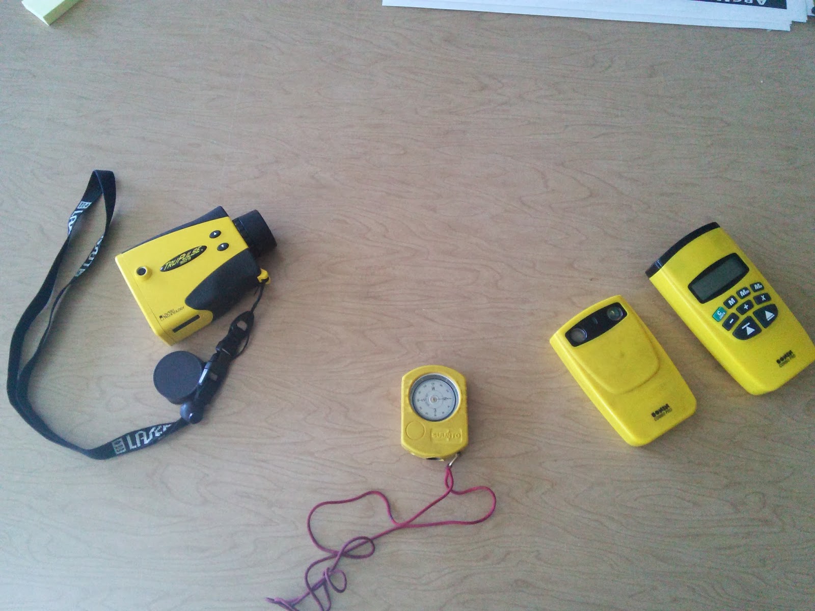
As mentioned in the Introduction, technology has progressed through the years; this applies to distance-azimuth surveying equipment as well. These technologies include a basic compass, a two-part radio range-finder, and a laser range-finder as seen in Figure 3.

The two part radio range-finder includes a receiver and a locator. The receiver is placed at the point of the object being measured while the range-finder is held at the point of origin. Once contact has been established between the two instruments. The locator will project both the distance (in meters) and azimuth (in degrees).

The laser range-finder is a much simpler, though more technologically advanced device. No receiver is needed, and the measurements are projected in a similar manner to the two-part radio range-finder.

Figure 3: From left to right, there is a laser rangefinder, compass, and two-part radio rangefinder. Each of these tools can be used to accomplish a distance azimuth survey.

In order to be prepared, all three of these tools were brought along. The initial plan was to use the two-part radio range-finder. Some complications were realized with this tool (which will be described later) and most of the survey was taken using the laser rangefinder.

Conducting the Survey

As mentioned in Instrumentation, the two part radio rangefinder was selected to conduct the survey. One member of our team would stand at the point of origin and call out distance and azimuth measurements while the other member would place the receiver at the point of every object to be surveyed and record the measurements and identification details (as seen in Figure 4)

. Figure 4: One member of our team is seen holding the receiver of the two-part radio range-finder. The other member, standing at the established point of origin would establish contact with the receiver using the range-finder to determine distance and azimuth measurements.

Establishing Point of Origin

The first step in actually carrying out the survey is to ascertain the point of origin for the selected location. Keep in mind, more than one point of origin may be used throughout depending on the needs of the survey. However, it is imperative to record the location of each point of origin. If distance and azimuth are not connected with the proper point of origin, any data and later mapping will be completely inaccurate.

The point of origin was established and recorded for the first of our intended four corners. Then, as previously stated, one member of our team "marked" each object with the receiver and recorded results while the other member manned the range-finder and called out distance and azimuth measurements.

Complications with Two-Part Radio Range-Finder
Before we had even finished surveying the first 25 points from the first point of origin, we realized that the two-part radio range-finder would not register any measurements beyond approx. 35 m. However, it was very good at establishing distance through thick foliage.

Switch to Laser Rang-finder
As a result of this complication, the decision was made to switch over to the laser range-finder (as seen in Figure 5). This instrument was capable of recording measurements of objects much further away. This eliminated the need for the data-recorder to also hold an instrument at the point of each object. In order to maintain detailed data, this member, instead, identified objects to be measured to ensure none were measured twice.

Figure 5: In this picture, a team member stands at the corner point of origin in Randall Park using a laser rang-finder to establish distance and azimuth measurements. A switch was necessary due to the limited range of the two-part radio range-finder

Challenges with Laser Range-Finder
While the laser range-finder could record measurements across much longer distances, it had trouble locating very thin objects such as telephone pole wires anchored to the ground. For very thin items it was necessary for the second member of our team to stand at the base of the object and to record the distance and azimuth by "shooting" the laser at the team-member.

In addition, it was less adept at shooting through other foliage, etc. After we had moved on to our second corner point of origin, it became clear we may need more than four points of origin at each corner of the park if we were going to collect approximately 100 points.

Point of Origin Adjustment
Faced with this realization, our initial plan was to establish two additional points on the edges of the park in-between the corners. After thinking this through a little more, a decision was made to shoot from the very center of the park.

This was the break-through decision for this project. Each corner of the park had only a limited path of vision to objects inside the park without obstructed views. By establishing a point of origin in the center of the park, we had opened up a 360 degree viewpoint with access to far more points than could be gathered from any of the four corners.

It became very clear we would not need to establish another point of origin to gather the necessary data. The remaining data points were gathered using the laser range-finder from a point of origin in the center of the park.

Data Entry
As specified, measurements were recorded in the field (as seen in Figure 6).

Figure 6: Distance, Azimuth, and Object ID data were recorded in the field to be placed in spreadsheets upon survey completion.

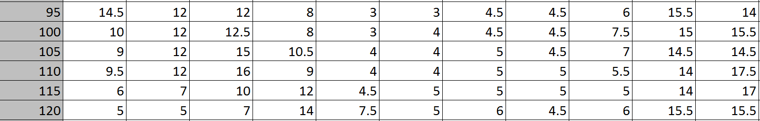
Data recorded in the field was simply transferred to Excel spreadsheets (as seen in Figure 7) allowing us to send it to ArcMAP to produce a visual of our results.

Figure 7: This figure shows the transfer of data taken in the field to Excel spreadsheets. The X and Y coordinates correspond with the point of origin information which was retrieved from ArcMAP once the information was transferred there.

Transfer to ArCMAP Geodatabase
After building a geodatabase specifically for this data-set in ArcMAP, the Excel Spreadsheets were imported to it. While object I.D.s such as "tree" or "bench" were recorded, the decision was made to omit their inclusion from the final map. It was not clear, with a diverse set of objects, how to appropriately differentiate them on any proceeding map.

To ensure the data was formatted correctly, the data layer containing our data-set was adjusted to the WGS 1984 Geographic Coordinate System due to the formulation of data based on latitude and longitude units. Failing to make this adjustment would have distorted our data presentation on the map. Also, it was necessary to include calculations for the points of origin to 6 decimal places. Just mis-recording information by .1 decimal degrees would translate to a land difference of approximately 8 km. and greatly reduce the accuracy of our map.

Visual consideration was also important. In order for readers to get a sense of the accuracy of our measurements and the area being surveyed an aerial imagery base map was added to the geodatabase.For this kind of a survey without any real focused purpose for selecting survey objects, this was the best way to convey our message.

Distance Bearing to Line Tool in ArcMAP
Continuing to work in ArcMAP, the Distance Bearing to Line tool was selected from ArcToolbox to build lines representing the distance, azimuth, and point of origin data (x and y coordinates) that had been collected and imported.

Figure 8: This figure displays the location of the Bearing Distance to Line tool found within ArcToolbox. This tool builds lines based on distance, azimuth, and reference point data collected in a survey.

Feature Vertices to Points Tool
Also found within Arc Toolbox the feature vertices to points tool (as seen in Figure 9) build a point at the end of each line built with the bearing distance to line tool. These points are representative of the "object" measurements were taken of.

Figure 9: This figure displays the location of the Feature Vertices to Points tool found within ArcToolbox. This tool establishes points at the ends of lines created using the Bearing Distance to Line tool. These points represent the objects measured.

Final Map

After employing these tools a final map needed just a few aesthetic touches before being displayed. In order to show the three different points of origin where data was taken from, the data originating from each point was differentiated by color (as seen in Figure 10). In addition, a title, legend, north arrow, and scale bar were added to help provide some context.

Figure 10: The final map produce in ArcMAP displays the distance/azimuth lines and points generated from our survey. Three colors were used to differentiate between the three different points of origin data was collected from.

Discussion

Field Adjustments

As is often the case with field work, the exercise required adjustment in the field. After collecting some data with the two-part radio range-finder it became evident it was not our best option for data collection. While it was excellent for establishing contact in obstructed areas, such as through foliage, the range of this was simply unsuited to the task at hand. 

Switching to the laser range-finder proved to be a wise decision even though it presented other challenges. The additional range we sought was worth making the switch. However, the laser range-finder was not nearly as good at sifting through foliage to make measurements, nor was it capable of identifying very thin items such as light pole wires. This was overcome by using the body of a team-member as the target for the range-finder.

As you can see in Figure 10, the range of measurements for our first two points of origin is rather limited. The yellow points' lack of range was mostly attributed to the two-part radio range-finder and its inability to record a measurement for more than 35 m. The second point of origin, in blue, had more to do with the inability of the laser range-finder to work around obstructions. 

What is clearly noticeable is the much wider paths, and longer distances recorded from the middle of the park. Our data collection time was greatly reduced by switching to this location. If the entire park were to be measured and not just 100 points (approximately), I would recommend beginning the survey from a point of origin in the center of the park. In addition, for accuracy, points of origin would need to be established in each of the four corners. This would ensure no features were missed.

ArcMAP Adjustments

It is imperative when setting the x, y coordinates in ArcMAP to record out to 6 decimal places (or more if you so choose). The misrepresentation of data on a map by rounding up or down will lead to a nearly illegible, unusable map. 

Also, we had originally included Object I.D. information (in the form of nominal data) to potentially make our map more clear. However, this information impacted where distance-azimuth line features were placed. When they were added, the placement of every line and point was moved to a different location. We are unsure of why this would take place, but either way, the information was omitted as a result.

Map Analyzation

It may not be clear unless you are looking for it, but there are definitely points on our map that do not line up with the points recorded in the field. On the far right of the map (as seen in Figure 10) there are lines going to points in the middle of the street. No data was recorded in these locations, rather they were taken in the boardwalk to the left of the street. It is uncertain why this misrepresentation of the data took place, but there are some possible explanations.  First, it could be the result of differentiation between the base map and coordinate system. There could have been shifting over time, though it seems unlikely to be that much. Secondly, in the midst of single-digit temperatures enhanced by sharp winds, it is possible that inaccurate measurements were recorded due to human error. Though we tried to account for any possible items we could possibly need in the field, it would have been ideal to employ a tripod to ensure steadiness while taking measurements. 

Conclusion

Distance-Azimuth surveying may be viewed as arcane with amazing tools like global positioning systems at our disposal. Still, having experience with fundamental surveying practices is extremely valuable. Even in the small sample of our survey, we ran into issues where technology was inadequate to record some types of results due to obstruction or distance. When the stakes are higher, the obstructions potentially larger, and the scope exponentially more broad, an infinite number of problems may arise. In order to be efficient in the field, having a repertoire of options is crucial. Simpler methods may not have the frills of newer technologies but by implementing a good strategy and adjusting to conditions, very accurate data can be collected using something like distance-azimuth surveying.

Field Activity #3: Unmanned Aerial System Mission Planning

Introduction

One of the most important aspects of unmanned aerial systems mission planning is the ability to assess the situation you have been given, develop a thorough plan, and communicate it to individuals and businesses that need to understand the process by which you will provide a solution for them.

• The mission plan should maximize productivity without endangering operators or equipment.
• In order to utilize the proper equipment, the mission plan should taken into account, weather, landscape, potential hazards, and the scope of the solution needed for clients.

Unmanned aerial systems (UAS) are typically divided into two broad categories, fixed-wing and rotary. In order to choose the correct UAS, you must understand their capabilities and limitations.

Fixed-Wing

A fixed-wing UAS (as seen in Figure 1) is capable of flight using wings that generate lift caused by the forward air-speed of the vehicle.

Figure 1: This picture provides an example of the size of a fixed-wing UAS. This particular model takes flight after being physically released by hand into the wind.

Flight Time: up to 26 hours              Speed: up to 175 mph              Payload: up to 350 lb.     

   

        Capabilities                                                                 Limitations

good for high altitude remote sensing                        limited ability to turn

long flight duration                                                     may require runway to launch or land
                                              
greater carrying capacity                                            inability to hover

high speed for greater coverage area                          limited close-up inspection capability   

Rotary

A rotary-wing UAS (as seen in Figure 2) uses lift generated by wings called rotor-blades (propellers) to revolve around a mast.

 

Figure 2: This picture provides an example of the size of a rotary wing UAS. For this particular model, four propellors revolve around masts propelling it into the air

Flight Time: up to 3 hours            Speed: up to 37 mph (approx.)            Payload: up to 75 lb.

       Capabilities                                                                        Limitations


vertical capability to hover and "stare"                                limited flight time

agile enough to come within feet of visual target                 limited payload

deliver payloads with precision                                           low operating speed

allows perfect camera pictures and angles                                               

each propeller can operate independently

not as effected by side-winds

good for facility inspections                       

more portable

vertical launch doesn't require runway

Mission Scenarios

This activity presents the following five scenarios. For each scenario we will provide a recommendation for how to configure the UAS and carry out a mission that will provide the required information to the concerned party.

Mission 1: Operation Desert Tortoise
A military testing range is having problems engaging in conducting its training exercises due to the presence of desert tortoises. They currently spend millions of dollars doing ground based surveys to find their burrows. They want to know if you, as the geographer can find a better solution with UAS.

Mission 2: Operation Power Tower
A power line company spends lots of money on a helicopter company monitoring and fixing problems on their line. One of the biggest costs is the helicopter having to fly up to these things just to see if there is a problem with the tower. Another issue is the cost of just figuring how to get things from the closest airport. 

Mission 3: Operation Healthy Pineapple
A pineapple plantation has about 8000 acres, and they want you to give them an idea of where they have vegetation that is not healthy, as well as help them out with when might be a good time to harvest.

Mission 4: Operation Leaky Pipe
An oil pipeline running through the Niger River delta is showing some signs of leaking. This is impacting both agriculture and loss of revenue to the company.

Mission 5: Operation Earth Removal
A mining company wants to get a better idea of the volume they remove each week. They don’t have the money for LiDAR, but want to engage in 3D analysis.

Mission Plans

For each of the five mission scenarios listed above, a mission plan has been developed. Each mission number and name will link back to the mission scenario for your review of the mission scenario.

Mission 1: Operation Desert Tortoise

In order to ascertain the needs of this mission we analyzed the following aspects:

1. The behavioral patterns of the desert tortoise and the geologic composition of their habitat 
2. The area coverage required for the mission 
3. The cost of current measures used to locate desert tortoises
4. The weather patterns affecting data collection
5. The equipment necessary to locate desert tortoises

Behavioral Patterns of the Desert Tortoise

Geologic Composition
The desert tortoise spends most of its life in burrows/shelters (as seen if figures 4-6) in order to regulate body temperature and reduce water loss. Sandy loam soils are the preferred location for these burrows/shelters due to their high resistance to flooding and high water holding capacity compared to other sandy soils. 

Figure 3: This is a pyramid explaining the different categorization of soils based on the quantity of silt, sand and clay it is composed of (states as a percentage). Sandy loam soil (outlined in red) consists of less than 7% clay, less than 50% silt, and between 43 and 50% sand. This soil is the preferred location for desert tortoise burrows.

Also, they are primarily found on the steep, rocky slopes of hillsides. The slopes may be littered with granitic or volcanic boulders and are often covered with dense vegetation. The palo verde-saguaro cactus is the most frequently occupied habitat, although some tortoises are found in oak woodlands and dense stands of bunch grass.

Vegetation
In addition, their burrows tend to be located in areas containing wildflowers such as wishbone bushes, lotus, loco weeds, spurges, blazing stars, lupines, Indian wheat, forget-me-nots, desert dandelions, gilias, phacelias, coreopsis, and many other species. They also eat annual and perennial grasses and fresh pads and buds of some species of cactus. They do not eat shrubs such as creosote bush and burro bush. 

Shelter Types
Shelters for the desert tortoise can be categorized into three different types based on the resources present on the landscape and the current needs of the tortoise. These three types are burrows, rock shelters, and pallets (as seen in Figures 4-6).

Burrow

Figure 4: Built into the side of a rocky slope, this burrow represents a "permanent" shelter for the desert tortoise used in all seasons. A burrow is typically between 2.5 and 10 feet in length.

    

Pallet 

Figure 5: This is an example of a pallet which equates to a "shallow" burrow that just barely covers the shell of the tortoise in spring, summer and fall. These temporary burrows or pallets use whatever cover is available in an area and can be fragile. They may be used for shelter for a few days while a tortoise is foraging in a particular area. A temporary burrow usually lasts from a few weeks to a season and disintegrates.

Rock Shelter

Figure 6: This is a rock shelter due to the composition of the material overhead as opposed to the sand/rock slope of the burrow in Figure 3. This is also a more permanent shelter for a desert tortoise.

Each tortoise usually has more than one burrow. In fact, desert tortoises may have between 5 and 25 burrows per year. The number of burrows the tortoise uses may depend on age and sex, as well as on the season. When burrows are constructed in soil, they are the size and shape of the tortoise -- half moon for the roof and flat on the bottom. Small tortoises have small burrows and large tortoises have large burrows.

Relevant Observations for Mission Planning
Based on these observations regarding the behavioral patterns of the desert tortoise our mission plan to locate desert tortoises will take into account the following geological and geographical features:

• Sandy Loam as the ideal soil for desert tortoise burrows
• The presence of vegetation such as grasses, wildflowers, and cacti as essential to the location of desert burrows due to dietary needs
• Tendency for shelters to be located along rocky slopes
• Variation of desert tortoise shelters into three categories - burrows, pallets and rock shelters

Coverage Area Required for Mission


While we have not been given information about the size of the military testing facility, based on the nature of operations at such a site, it is safe to assume a wide coverage area. Collecting data from a large circumferential area will require an unmanned aerial system with long flight range. It will also be preferential for the UAS to be capable of high speeds to complete a mission of this magnitude in a reasonable amount of time.

With a coverage area of this scope, it is important to make use of ground control points. Ground control points are points on the surface of known location. These locations are normally found by measuring the coordinates using a GPS. These points will allow us to geo-reference the image during post mission analysis.

Cost of Current Methods for Locating Desert Tortoises

From the information we have been supplied, the cost of locating desert tortoises currently is in the millions of dollars. Every time military testing takes place, data must be collected and desert tortoise location determined. Due to the high costs associated with such an endeavor options such as LiDAR remote sensing technology and high resolution photography equipment should be considered if additional precision can be gained through their use.

Weather Patterns Affecting Data Collection

Every time that military testing takes place, it is required that the location of all desert tortoises be determined. Because desert tortoises will have between 5 and 25 burrows that, potentially, vary from year to year, data collection will take place on a regular basis. As such, weather is not a long-term consideration. Data collection will take place subject to the needs of the military testing facility as opposed to the ideal long-term timing of data collectors such as seasonal considerations.

However, in the short-term, the absence of factors such as rain, strong winds, and low visibility conditions will be required for the accurate collection of data.

Equipment Options for Data Collection
This section will be used to present the abilities of equipment options available for accurate data collection based on the details of this project. How they will be used will be discussed in the Mission Plan.

This will include unmanned aerial system options as well as sensors, cameras, GPS units, or other data collection options recommended.

Unmanned Aerial System
Fixed-Wing Aircraft

Falcon Eye fixed-wing UAV
A fixed-wing UAS (as seen in Figure 1) is capable of flight using wings that generate lift caused by the forward air-speed of the vehicle.

Figure 7:This is a picture of the Falcon Eye fixed-wing UAS . This particular model requires a runway for launch. 

                               Flight Time: up to 24 hours                  Speed: up to 112 mph   

Cruising Altitude: up to 18000 ft.         Payload: up to 220 lb.     

   

        Capabilities                                                                 Limitations

good for high altitude remote sensing                         limited ability to turn

long flight duration                                                     may require runway to launch or land
                                              
greater carrying capacity                                            inability to hover

high speed for greater coverage area                          limited close-up inspection capability


Reasons for Selecting this UAS
Due to the significant coverage area required to collect data from, a fixed wing UAS, such as the Falcon Eye will be necessary. Whereas rotary UAS models only have up to 3 hours of flight time, this fixed-wing aircraft will allow up to 24 hours of flight time for data collection. In addition, at a speed of 112 mph, the Falcon Eye will be able to collect data in a reasonable amount of time. Because data collection will take place at a military testing facility, it is understood that a runway will be available.

Hyperspectral Imaging Sensor

A hyperspectral imaging sensor (as seen in Figure 8) collects and processes information from across the electromagnetic spectrum.

Figure 8: This image is a hyperspectral imaging sensor. It will be mounted onto our fixed-wing UAS to provide data by remotely sensing the surface of the Earth in our study area. This information will guide us to the location of various types of soils and vegetation for identifying the location of desert tortoise burrows.

The hyperspectral imaging sensor divides light into many bands including the visible spectrum and those beyond the range of the human eye including infrared, ultraviolet, etc. (as seen in Figure 9).

Figure 9: This is a diagram of the bands of the electromagnetic spectrum as viewed by hyperspectral imaging sensors. As stated on the diagram, vegetation can be differentiated in the Red Band of the spectrum. Soil types can be discriminated in the Longwave Infrared Band. Using the hyperspectral signature attached to the soil and vegetation types we are looking for, we will be able to locate potential desert tortoise burrows.

Using visual images obtained by the hyperspectral imaging sensor, the red band will allow us to identify the vegetation associated with desert tortoise burrows. In addition, the longwave infrared band will allow us to establish the location of sandy loam soil throughout the region in question.This soil type is the typical location of desert tortoise burrows. These features are easily identified because each type of soil, vegetation, etc. has been cataloged with a specific spectral signature based on the amount of light (energy) reflected. These signatures are read on a chart produced from information gathered by the hyperspectral sensor (as seen in Figures 10 and 11)

Figure 10: This chart shows how different features such as grass, soil, and water reflect different percentages of light and thus can be identified. By locating specific areas of vegetation we will be able to narrow down the potential locations of desert tortoises.

Figure 11: This chart shows the reflectance patterns specific to Sandy Loam variations. Through hyperspectral remote sensing, the location of all sandy loam in the area in question will be located for the identification of desert tortoise burrows.

Post Mission Analysis

Aerial images taken during the mission will be imported into a remote sensing program in which the desired spectral signatures can be measured, identified and differentiated. Using our predetermined ground control points, we can anchor down certain locations on the aerial imagery in order to establish a coordinate system. Once these signatures have been located, the images can then be imported and projected into a GIS in order to find the coordinates of potential desert tortoise habitats.

***ADJUSTMENT TO CURRENT FORMAT***

The extent of this mission planning exercise has been exceeded as far as what you see in mission 1. As a result my instructor has advised providing only the essential details as far as what sensors, UAS, and other equipment recommended to complete the mission.

Mission 2: Operation Power Tower

For Operation Power Tower, a UAS is needed to examine various power lines and electrical towers. We decided that a rotary UAS will be the preferred method in order to hover and stare at various components on each electrical power. A small high resolution camera will be mounted onto the UAS in order to provide a live video feed to the pilot and concerned party. UAS mission planning software will be used to set predetermined stops at each tower to minimize flight time and maximize mission efficiency due to the short battery life of the rotary UAS.

Mission 3: Operation Healthy Pineapple

Operation Healthy Pineapple required an analysis on the health of a large scale pineapple plantation. Because this mission will be covering a distance of 8000 acres, it calls for a long flight duration and high altitude, which makes a fixed wing UAS the ideal vehicle. In order to measure the health of the pineapple, a multispectral sensor will be mounted to the UAS. This sensor will allow us to examine the different spectral signatures found within the red band of the visible spectrum to identify healthy pineapple and unhealthy pineapple. 

To determine the optimal harvest time for pineapple, it is recommended that multiple data collection runs be made over the course of the standard harvesting season. 

Mission 4: Operation Leaky Pipe

Operation Leaky Pipe involves locating the source of oil pollution within the Niger River Delta. To find this information, we will be using a two stage process including two different UAS vehicles. The first stage of the mission will require a fixed wing UAS equipped with a hyperspectral scanner to locate areas of oil pollution in the river delta using the green band of the visible spectrum and potential areas of impacted crops using the red band. By using remote sensing software, areas with these spectral signatures will be located in the river delta until the furthest location of pollution upriver is found. 

In the second stage of the mission a rotary UAS will hover to the upriver location identified by the fixed wing UAS. The rotary UAS will be equipped with a small high resolution camera which will provide a live feed to the pilot and concerned parties and a GPS unit in order to locate the oil leak. Locating the oil leak will also help us understand the scope of crop damage than can be attributed to the oil leak as opposed to damaged crops further upstream. 

Mission 5: Operation Earth Removal

Operation Earth Removal required volumetric analysis in order to measure the amount of material removed from the mine each day. Using a rotary UAS will allow us to adjust the vehicle until we find the desired elevation and angles that will provide the most accurate measurements to calculate volumetric output. At the end of each workday, the UAS will fly over the mine and generate point cloud data using a point cloud sensor. Point cloud data can be used to generate a 3D representation of the mine, which can be compared to the mine measurements of the previous day to determine the difference in volume.

Field Activity #2: Visualizing and Refining Terrain Survey

Introduction:

Emphasis
Field Activity #2 emphasizes assessing the viability of various surface terrain models, determining accuracy of sampling methods, and resurveying. Digital terrain models (DTMs) are used to turn data points into a visual displaying the basic terrain profile per the measurements obtained. Per the instructions below these various models will be displayed, compared, and contrasted in general. In addition, their applicability for the box plot survey from Exercise 1 will be examined.

Instructions

1. Import the XYZ table developed in Field Activity #1 to ArcMAP and make it into a point feature class.
2. Turn the point feature class into a continuous surface.
3. Develop terrain profiles using the following interpolation methods:
• IDW
• Natural Neighbors
• Kriging
• Spline
• TIN
4. Discuss advantages, disadvantages, and observations regarding the 'fit' of each interpolation method.
5. Determine which method best fits the survey

Methods:

Building Initial Terrain Profile
The XYZ table developed in Field Activity #1 was imported as a layer into ArcMAP in order to create a point feature class. Next, this point feature class needed to be displayed to ensure that the points were consistent with what had been collected in the field during our box plot measurement. By using the "Display X,Y data" tool, the points that we had measured could be visualized (as seen in Figure 1). This grid represents all the data points collected. As you can see, the data entered appears to have been displayed consistently with even rows representing the measurement intervals employed in the field.

Because the box plot was merely a model of terrain, no specific projection needed to be applied to this data set.

Figure 1: This figure is the X,Y data points collected from the box plot. These measurements were taken at intervals, thus the points are in even rows throughout. 

Exporting File as Geodatabase
Based on the experience of my fellow students, I initially tried to export my file as a "shapefile". After consulting with several students and my professor, I was still not able to develop the models properly. It was advised that I export my file as a geodatabase (gdb). After doing this, I was finally able to develop the five digital terrain models (DTMs) as specified in this exercise.

Development of Digital Elevation Models in ArcScene

The interpolation process that turns the data points in Figure 1 into the following models is essentially "filling in the gaps" between the points in order to display a continuous surface. Without this process, all that would be displayed would be the elevation measurements at each point. This would in no way resemble the actual surface from which measurements were taken. By smoothing out the areas between measurements, a visualization can be developed to give someone a more accurate representation of an actual surface.

Difficulties
I have initially run into complications trying to to develop the terrain profiles using interpolation methods. Because I am just now taking a GIS class, I am very uncertain of the steps involved. After learning about how to import the XYZ table, turn it into a point feature class, and develop terrain profiles, I tried to carry out the process unsuccessfully. Over the course of two days, I sought  the advice of my peers who walked me through the process step-by-step. Even after seeking help, much to the consternation of those who assisted me, I was still not able to build these terrain profiles.

Assessment of Generated Profiles
After viewing the basic elevation profile based on our XYZ, we were able to locate areas where our measurements may be off. Looking at the profile together, we determined the areas where we would potentially want to resurvey as seen in Figure 1.

(Figure will be inserted with the completion of my profiles)

Re-examination of Physical Terrain
Next, we brought our profile out to our garden planter box to compare with the actual physical terrain.We also brought with us our initially recorded data. By comparing the two, we solidified are choices for resurvey as a group. Then, we plotted our areas to be resurveyed on our initial data set.

Determination of Re-Survey Methods
While still outside, we discussed how we would improve upon our initial survey. The decision was made to divide the identified grids for resurvey into four 2.5 x 2.5 cm grids. In order to avoid confusion, we also decided to use a different color string for the additional grid divisions.

Additional Grid Construction
Following the methods employed in Field Activity #1, we built the additional grid lines with thumbtacks and pink string as seen in Figure 2. In order to ensure accuracy, one member of our group guided the placement of each new grid line based on the plotting we had added to our initial survey.

Figure 2: Original grid squares were divided into four 2.5 x 2.5 cm. grids for re-survey

Re-Survey Process
During our initial survey, the 5 x 5 cm. grids were fairly easy to keep track of and measure. This became much more difficult with the 2.5 x 2.5 cm. grids.

• First, we realized that an original meter stick would be too wide to fit into the smaller grids and had to go get a thinner one.
• Second, it was not as simple as identifying the southwest corner of each grid. In order to provide accurate information to the person recording the data we had to identify a pattern for measuring the four grids that had previously been just one.
• Third, because of the smaller area, it became necessary to place a meter stick along the top of the grid to provide support in order to limit the amount of movement as we measured.

(*these additional measures are shown in figure 3.)



Figure 3: A meter stick was placed along the top of the grid to stabilize for measurement and a thin meter stick was used to take measurements in the smaller grids

After carrying out this res-survey process, the steps to enter data into ArcMAP in order to generate the DEMs was gone through again. Now, I will develop these models to asses there accuracy at displaying our actual box plot surface.

Triangulated Irregular Network (TIN)

For a TIN, a set of points is combined with elevation measurements to create "triangles" with all of the data points collected being located in the corner of the triangle.Each triangle is completely separate from every other triangle, thus there is no overlap. Because of this process a TIN is best for visualizing points in an irregular pattern.

The nature of the features developed in our box plot had far more regularity than regularity, so the TIN is not really the best option for displaying our data points. That being said, to understand the general layout of our box plot, a TIN does a reasonable job (as seen in Figure 4). It is clear to see where the areas of height and depression are located, etc.

Figure 4: This TIN representation of our box plot makes it easy to interpret the general layout of our box plot.

However, when look at from a more "straight-on" view (as seen in Figure 5), many of the peaks are displayed much more sharply than the actual features they represent. This is the result of the triangulation process for interpreting the data. throughout the image, you can see the various triangles for each point making it seem like there is much more variation throughout the surface than there actually is.

Figure 5: This more straight on view of a TIN surface projection makes the triangle-shaped points for each data point much more evident. This is not an accurate representation of our data which is far less sharp and much more even.

Inverse Distance Weighted (IDW)

This interpolation method determines cell values for each data point using a "linearly weighted combination of a set of sample points". With this method, the assumption is that the influence of the variable being mapped decreases with distance. This results in each data point "clumping" in one spot rather than evening out the area between data points (as seen in Figure 6). The surface is basically pock-marked with the data points especially where there is a difference in elevation. In areas where there is no variability in the height measurement the data appears very even. This is probably abnormally even.

Figure 6: This figure shows represents our box plot using the IDW interpolation method. This method assumed influence of a variable decreases with distance. Thus data point height measurements are clumped around the data point rather than smoothed from point to point.

Once again, the more straight-on view of this interpolation method shows abnormally differentiated peaks (as seen in Figure 7). There are not the harsh edges of the TIN method, but the data points still stand out unreasonably compared to the actual surface.

Figure 7: While the peaks are not as sharp as seen using the TIN method, they are still overly pronounced when compared to the actual surface due to the method of decreasing influence away from the data point employed in the IDW interpolation.

Kriging

The Kriging interpolation method generates an estimated surface from a scattered set of points with z-values. It is based on statistical models that employ autocorrelation. In other words, they take into consideration the surrounding measured values and mathematically determine the smoothness of the resulting surface. This smoothing process results in a much more even surface (as seen in Figure 8). Gone are most of the bumps and sharpness seen in both the IDW and TIN interpolations. This makes it a little more dificult to differentiate the surface overall, but this is actually more accurate to the actual surface.

Figure 8: Using the Kriging method results in a much more smooth representation of the actual surface it represents. 

However, when viewed straight-on, the height differentiation throughout the surface is actually very clear (as seen in Figure 9). There are noticeable peaks on the back edge that do not correspond with actual data from our box plot. This is a point of concern. This views is an especially good representation of our actual data.

Figure 9: The straight-on view of the Kriging Method is very smooth, and height differences are very clear as well. This is a very good representation of the data from our box plot.

Natural Neighbor

The Natural Neighbor interpolation method finds the closest subset of input samples to a query point and applies weights to them based on proportionate areas to interpolate a value. Basically it estimates the slope between points and, based on that, determines the height of the points. This results in a very smooth representation of the data (as seen in Figure 10). However, compare to the Kriging method some areas tend to get amorphous and lose their definition altogether such as in the foreground (in green).

Figure 10: This representation of the data using the Natural Neighbor method offers a very smooth display, thus the term "natural" in the name.

The straight-on view of the Natural Neighbors method is also very smooth with the unexplained spike in the background (as seen in Figure 11).  The elevation points are a little bit sharper than seen using the Kriging method. A determination must be made as to which view is a more accurate representation of the data

Figure 11: This straight-on view of the Natural Neigbors interpolation offers a very smooth surface only slightly more sharp than the Kriging method.

Spline

The Spline interpolation method estimates values using a mathematical function meant to minimize overall surface curvature, resulting in a smooth surface that passes exactly through the input points. The resulting surface will minimize any sharp features in the data. It is best used for gently varying surfaces such as elevation, water table heights, and pollution concentrations. As seen in Figure 12, the surface appears almost flattened out. Whereas the IDW and TIN methods overstated peaks, this method has underestimated them. 

Figure 12: Using the Spline Method, sharp features such as peaks are minimized resulting in a flattened out representation of our box plot.

Looking at the Spline interpolation straight on, actually shows a fairly nice representation of our data. Even the unexplained sharp peak in the background is minimized here (as seen in Figure 10). It may flatten out some of the peaked areas, but seen from this view, it gives a really good sense of our box plot.

Figure 12:  The straight-on view of the Spline interpolation method shows minimized peaks, but is an overall fair representation of our actual box plot.

Discussion:

Due to the over-pronounced peaks seen in both the TIN and IDW models, I do not believe they are the best option for displaying the box plot data. The nature of this surface just wasn't irregular enough to make these the most useful methods.

When viewed straight-on, I feel that Kriging, Natural Neighbors, and Spline all do a very nice job representing the box plot. However, when comparing them to each other Kriging still shows peaks being less-sharp than does the Natural Neighbors method.

In addition, the Spline method really does a nice job softening the peaks of our surface. At first, I thought it perhaps rounded out our peaks too much but now actually think this is more accurate than any representation showing sharp features. We just didn't have any very sharp features on our surface. This method is stated to be good for displaying elevation as well. Due to these aspects, I recommend the Spline method for displaying the data from our box plot.

It is quite possible we should have gone over our data more thoroughly and eliminated the unreasonable points such as the peak in the background in the straight-on view using any of the interpolations.

Conclusion:

Assessment of Methods
Throughout Field Activities 1 and 2, our group hoped to build on the experiences of the Field Methods class from 2013. Thus, we immediately employed 5 x 5 cm. intervals, built our elevation using the top of the garden planter box, and discussed our plans thoroughly before implementation.

In order to try improve upon our initial data results, we chose to measure smaller grids to try to better capture the change in elevation in areas we found to be misrepresented in our initial terrain profile.

As we went along, we also became more adept at asking questions regarding our process. Why, how, where, and when may seem trivial, but they were critical questions to address for every step of the process. That way, when the time came to record our experience, it would not just be a guessing game.

Areas for Improvement
Were I to undertake this experiment again, I would do the following:

• designate an official note-taker to fastidiously record not only the details of what we did, , but what we were thinking and why, conditions that were influential, and questions to consider later
• do a more thorough job looking at previous experiments - after the fact I learned that a group last year had used a spray bottle to freeze their terrain surface. As you can see in figure 13, our terrain is checkered with meter stick markings that, no doubt, led to some misrepresentation of the actual elevation of our features.

Figure 13: Our terrain is covered with "incisions" from where the meter stick contacted the terrain surface

• determine whether or not using a range finder would be an option - spraying the surface to freeze it would not be necessary if we could measure elevation without physically touching the terrain
• double and triple check the data set for any possible aberrations leading to obviously wrong data points

Group Assessment
As someone who insists on being thorough, I could not have asked for a better group to work with than John, Emily, and Carolyn and Brendan. Every time we worked together, everyone pitched in unreservedly. Spending the time in planning, preparation, and asking the right questions with one another made it so much easier to record the progression of this experiment. Being someone who has almost no GIS experience, one group member in particular (John) went far out of his way to try and guide me through the process. I would choose to work with this group again if given the opportunity.

Personal Learning Outcomes
I must refer back to my conclusion from Field Activity #1 to explain my learning outcomes which are as follows:

• Assess and plan properly
• Be fluid and creative
• Reflect and learn
• Move Forward

All of the little details of performing a GIS operation, or laying out a measurement grid are merely memorization functions. What separates a person is taking the time to prepare and analyze, think and ask questions, bounce ideas off of one another, reflect on your experiences in order to learn, and make plans for how to adjust in the future.

To be good in the field requires being observant, patient, resourceful, and careful. The integrity of the data you collect will be at the mercy of these elements far more than the technical machinery and methods you employ to obtain them.

Field Activity #1: Creation of a Digital Elevation Surface

Introduction:

Emphasis

Field Activity #1 emphasizes critical thinking skills and the ability to implement improvised
survey techniques.

Instructions

1. Construct an elevation surface of terrain in a garden planter box (See Figure 1) including the following terrain types.
• Ridge
• Hill
• Depression
• Valley 
• Plain
2. Survey the elevation surface with rudimentary tools such as a measuring type and meter stick.
3. Record the results of the survey in a spreadsheet containing X, Y, and Z fields for later entry in ArcGIS.

Figure 1: Garden planter box in which we were to build our elevation surface



Methods:

Elevation Surface Construction

"Snow or Sand?"
As you can see in Figure 1, January and February, 2014 provided us with an ample amount of snow. That and the cold temperatures made it an easy decision to construct our elevation surface out of snow rather than the rock solid sand beneath it.

"Build up or Down?"
Next we had to decide whether to build "up" or "down." At first, the large amount of snow made it seem like it would be easiest to build up from the top board enclosure of the planter box and use the enclosure as the base-level. However, we felt that this would lead to imprecise measurements if we were trying to determine the height of that outer edge when we were measuring in the middle of the planter. We concluded it would be best to use the top edge of the enclosure as our maximum height. This meant we would measure down from the top to determine the elevation profile.

Physical Feature Placement
The actual construction of our six terrain types required us to get our hands dirty (or, at least, cold) as can be seen in Figure 2. We did our best to recall our Geography 104 (Physical Geography) course in order to place features where you would typically expect them to be.



Figure 2: Physical construction of the elevation surface



Terrain Survey

Equipment Selection 
After studying the methods used in the Geographic Field Methods class from 2013, we decided to use push pins and string to develop a grid system from which to taken measurements.

Interval Selection
Again, building on the work from Geographic Field Methods - 2013, we noticed that some of the groups initially started with 10x10 cm. grid squares. Later they wished they had used smaller intervals. Therefore, we decided to start with 5x5 cm. grids in hopes of avoiding a re-survey.

Grid Construction
Armed with our selected intervals, we used a meter stick to mark our 5 cm. intervals around the enclosure board of the garden planter box as seen in Figure 3.

Figure 3: Push pins were used to mark 5 cm. increments on the outer edge of the garden planter box

 Next, we divided the area of our garden planter box by running string across the box at our 5 cm. intervals until we arrived out our finished project as seen in Figures 4-6.

 

Figure 4: String was extended from corresponding 5 cm. increment pins to create our grid structure

 

 Figure 5: View of string extension across the garden planter box

 

 

Figure 6: Final 5x5 cm. grid pattern view from the top 

Terrain Elevation Measurement

Logistics
As previously mentioned, our next step was to measure down from the top of the grids to the terrain beneath. In order to ensure consistent measurement, we measured from the "southwest" corner of each grid using a meter stick. Because we were dealing with a hypothetical terrain. We chose our north, south, east, and west directions without regard to actual direction. Figure 7 is labeled with the direction we chose for north

 

North

Figure 7: North is labeled at the top of this photo. Measurements were taken from the southwest corner of each grid.



Figure 8: Using a meter stick, measurements were taken from the top of the grid to the height of the surface below at the southwest corner of each grid

 

Measurement Process
Every precaution was taken to ensure accurate measurements in spite of the less than ideal methods available to us. As seen in figure 9, one person measured distance from the top of the grid to the elevation height below, one person stabilized the meter stick in the southwest corner of the grid, and a third person called out measurements from an eye-level perspective of the top of the grid. A fourth person (not in picture) recorded the measurements in a pre-made grid diagram.

 



 Figure 9: Ensuring accurate measurement, one person measured the height of elevation, one person stabilized the measurement location in the southwest corner, and one person called out the measurement to be recorded

 

 

 

Adjustments

As we took our measurements, we noticed the grid lines we had placed were not always tight. In order to account for the effect of this on our measurements we rounded them to the nearest half centimeter. 

Data Entry of Results

Matters of Interpretation

Armed with the results of our survey, we undertook the painstaking process of entering our data into a Microsoft Excel spreadsheet as seen in image . At first, this might seem mind-numbing, but we soon realized this would take a little bit of thought. Two different people added the raw data; one recorded positive numbers, and the other recorded negative numbers as is shown in graph 1. This meant we had to re-format our data.

 

 

      Graph 1: original entry of elevation measurements from the top of the grid with some positive and some negative numbers from two people's interpretation of the data. The grey column corresponds with the data row.

 

 

Establishing "sea-level"

Before doing so, we also had to set a "sea-level" because we were taking measurements from the top down to terrain elevation. By looking at our results, we saw that the lowest measurement recorded was 20 cm. This became our hypothetical sea-level. Using that sea level, our measurements from the top of the grid were reformulated to show height from sea level as seen in Graph 2.

 

 

 

Graph 2: Reformulated data shows all positive values as measure "up" from 20 cm depth (sea-level) to the top of our grid as opposed to positive and negative measurements "down" from the top of the grid..

 

 

Translation to X,Y, Z coordinates

The final step of our data entry was to take our pre-survey grid with numbered x and y coordinates and combine them with our measured z coordinates in an excel table as seen in graph 3.

 

 

Graph 3: This is the translation of our grid data points into X, Y, and Z coordinates for future entry into ArcMAP

 

 

Discussion/Conclusion:

(Due to the detailed nature of the Methods section and the relative lack of results associated with the first portion of this exercise, I have combined these two sections into 1.)

 

Overview

 

This exercise presented some very unique challenges in all three steps (elevation surface construction, terrain elevation measurement, and data entry of results) of the process. It truly showed the intentional manner in which decisions must be made while doing field work in order to ensure the accuracy, precision, and consistency of data collected.

 

Assess and Plan Properly

     

More important than the "doing" of fieldwork is the development of your methods and the reasons for them. Assessing the situation and developing a solid plan prepares allows you to address the variability you will inevitably encounter in the field. Fortunately, the group I worked with saw the value of these measures and stuck to them.

 

Be Fluid and Creative

     

I can definitely see how electronic measures to ascertain the elevation profile of our garden planter box. However, I can also the value in being able to creatively develop solutions without ideal tools.  

 

Reflect and Learn

     

There were times where our group created extra work by failing to talk things through. For instance, the data points being entered in positive and negative numbers was a small hiccup.

 

Second, we noticed that the accuracy of our height measurements many have suffered as a result of an inadequately tight grid line. We tried to account for this by rounding our height measurements to the nearest half-centimeter, but there is more room for error in this generalization.

 

Thirdly, we should have devised a way to better keep track of our directional choice of N, S, E, and W. We often had to regain our bearings by asking, "which way is north, again?" when entering data.

 

Moving Forward

     

In the next portion of this exercise, my group and I will be assessing the results of our initial survey. Then, we will make any necessary changes to our data based on what we have found. From there, using ArcGIS, we will develop different models displaying our elevation profile and determine which one best expresses our data.